
Your Chance to Feature Planet Hunters on the Daily Zooniverse
Each day something new from across all the Zooniverse projects is featured on the Daily Zooniverse blog organized by the Zooniverse’s Grant Miller. Have you classified a weird light curve or participated in an interesting discussion on Talk? Now’s the chance to have that highlighted on the Daily Zooniverse. Grant and the Daily Zoonvierse team are looking for contributions from the volunteers of Zooniverse projects (including Planet Hunters) to feature. Just add the hashtag #dailyzoo to a light curve or discussion page on Talk to nominate it.
If you want to also share your nominations with the rest of the Planet Hunters community, there is a thread started on Talk where you can can list your finds for everyone to see (do make sure to include the hashtag). If you’re looking for inspiration Echo-lily-mai, one of our Planet Hunters Talk moderators, has nominated this folded light curve plot of a candidate heartbeat star made by volunteer Sean63 :
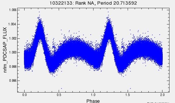
Image Credit: Sean63/Planet Hunters
Studying the Chemistry in Protoplanetary Disks (Part 2)
Today we have a guest post from Colette Salyk. Colette is the Leo Goldberg Postdoctoral Fellow at the National Optical Astronomy Observatory in Tucson, Arizona. She studies the evolution and chemistry of protoplanetary disks (the birthplace of planets) using a variety of ground and space-based telescopes.
Welcome to Part II of my three-part post about studying the chemistry in protoplanetary disks! (You can find Part I here.) In the last post I talked about techniques for detecting molecules. But once we detect them, what do we do with these detections? Ultimately, we want to make chemical “maps” of the protoplanetary disks, so we can understand what kinds of environments planets are forming in at different distances from their host star. In this post I’ll explain how we use the Doppler shift (yet again!) plus Kepler’s law to locate molecules in protoplanetary disks. (In Part III, I’ll discuss some of the connections between disk chemistry and the formation of planets.)
In the figure below, I’ve reproduced the observed water emission line that I discussed in my first post, but have converted wavelength to velocity using the Doppler shift equation, (λ−λ0)/λ0 = v/c , and centered the line at zero velocity. Note that in the first post, I focused on the shift of the entire line relative to the theoretical line center; here I am repositioning the line to account for this new center, and we’ll be discussing Doppler shifts relative to this new center.
 Although molecules emit/absorb at very specific wavelengths, the water vapor emission line we observed is clearly not thin and pointy. Instead, it has a rounded shape — something we refer to as “line broadening.” This broadening occurs for all spectra, due to two reasons. One reason is that the instrument optics always blur out the signal somewhat — this is called the “instrument response function.” The other reason is that the molecules themselves are always moving, and the motion of each molecule produces a Doppler shift. Collectively, they produce emission at a range of wavelengths. In our case, the instrument response function (plotted in the figure) is much narrower than our line. Therefore, the broadening is dominated by the motion of the molecules.
The molecules are moving around due to a variety of reasons, including bouncing around due to their temperature, being kicked around by turbulence, and being in orbit around the star. The last effect dominates in our case, and I’m going to focus on that motion in this post. A simple example that may help you picture how orbital motion broadens the emission line is to consider a thin ring of molecules orbiting a star, oriented edge-on to our view. The molecules on one side of the star are moving away from us, and are redshifted; the molecules on the other side are moving towards us and are blueshifted. The amount of Doppler shift also depends on the orientation of the motion — as we examine parts of the ring that appear “closer” to the star from our point of view, we see progressively more transerve motion, and progressively less radial (and therefore Doppler shift-producing) motion. This collection of Doppler shifts turns a thin theoretical emission line into something broader, with symmetric blueshifted and redshifted components.
How fast are the molecules moving in the disk as they orbit their host star? If you’ve taken Astronomy 101, you’ve probably heard of Kepler’s laws — they are a set of relatively simple rules that dictate how the planets of the solar system orbit around the sun. Kepler’s third law relates the period (P) and semi-major axis (a) of planetary orbits, stating that P^2 ∝ a^3. Alternatively, astronomers often convert period to velocity (using v = 2πa/P), and put in the correct constants so that the law applies to stars of all masses (not just ones like the sun), to obtain: v = sqrt(GM⋆/a), where G is the gravitational constant and M⋆ is the mass of the star. This is a very powerful statement, because it means that we can directly relate velocity (v) to distance from the star (a). Since we can use the Doppler shift to measure velocity, we can therefore use the line broadening to measure the location of the molecules.
In contrast to the simple ring example I gave above, real emission lines originate from a range of disk radii, and the amount of light emitted at each radius also depends on the temperature and density of molecules. Also, the line width depends on how inclined the disk is with respect to our view. The figure below shows example emission lines originating from a disk where I’ve assumed the molecules are located between two radii, Rin and Rout, and that the disk is inclined by 30°. Have a look at the plots to see how the line shape depends on both Rin and Rout.
 What I find especially cool about this technique is that it works especially well when the molecules are at small radii. For example, it’s really easy to tell the difference between molecules located at 0.1 AU vs. molecules located at 1 AU! It’s not currently possible to obtain this kind of detailed spatial information through imaging alone, and so we sometimes say that we’re achieving “super-resolution”. I think this is a neat parallel to the Kepler mission, in which the transit observations are used to obtain detailed information about the sizes and orbital radii of planets, even though we cannot directly image the planets.
Now some questions for you. Have a look at the detected water emission line in the first figure. Assuming this disk is inclined by 30°, as I assumed in my models, where do you think the molecules are located in this disk?
Latest Science Paper Accepted for Publication: The First Kepler Seven Planet Candidate System and 13 Other Planet Candidates from the Kepler Archival Data
Today we have a post from Joey Schmitt, a graduate student in the Astronomy department at Yale University, where he is working with the exoplanet group led by Debra Fischer, and in particular he has been working on the follow-up of Planet Hunters planet candidates.
We at Planet Hunters are happy to announce the acceptance of the PHVI paper to the Astronomical Journal, in which 14 new planet candidates were discovered. All of these new planet candidates are located far from their host stars. In fact, seven of them lie in their host star’s habitable zone. Unfortunately, all of these planets are too large to be Earth-like.
Two of the new planet candidates are in multiple candidate systems. One of them, the new candidate orbiting KOI-351, is the seventh planet candidate orbiting its host star. Planet Hunters actually detected three new candidates around this star when KOI-351 was only known to have three candidates, showing how great the Planet Hunters can be in discovering multiple planet systems. The planets in KOI-351 also show strong gravitational interactions between the planets, which helps to confirm them as true planets. The gravity from some planets in the system causes other planets to transit before or after what we would otherwise expect, called transit timing variations. In fact, the second-to-last planet transited a full day after we expected it would. Others in the exoplanet field have been working for over a year to determine the masses of these planets.
The new candidate in KOI-351 makes it the only star with seven known transiting planets. After our submission in October, two other teams claimed confirmation of the seven signals to various levels of certainty. Look forward to the brand new stars in the K2 campaign, changes to the Planet Hunters strategy, and new papers of the latest planets and candidates discovered by Planet Hunters.
You can read the revised accepted version of the paper here. The Planet Hunters volunteers who participated in identifying and analyzing the candidates presented in this paper are acknowledged at http://www.planethunters.org/PH6, and the contributions of the entire Planet Hunters community are individually acknowledged at http://www.planethunters.org/authors.
