
Planet Hunters NGTS: More detail on our first four Planet Candidates
You may have seen my previous post announcing that we have 4 new planet candidates discovered by Planet Hunters NGTS, if not you can find it here. We wanted to give you some more information on what we know about each candidate so far and the efforts we’ve made to gather follow-up data as we work towards ascertaining whether or not they’re real exoplanets! The first step once we decided that these candidates were worthy of further investigation was to fit the data using a more intricate model. This is typically what’s meant by phrases like “modelling estimates” or “fit results” that you may see below or in other pieces of science communication. Each of these candidates pose their own unique challenges in being able to confirm whether they’re really planets, however to already have 4 planet candidates is a promising sign for the future of the project and a real testament to the brilliant work put in by you, the Planet Hunters NGTS volunteers.
Subject 69695263: This is our most promising candidate so far as the transits look quite clear and our modelling estimates give encouraging results. We think this is a hot Jupiter orbiting a “K dwarf star,” which is a star slightly smaller and cooler than our Sun. We’ve estimated that the planet candidate has a radius equal to 1.09 times the radius of Jupiter, which we write as Rp=1.09 RJup. It orbits its host star every 1.74 days which means by the time you turn 18 Earth-years-old, you’d be almost 3800 years-old on this planet candidate (if it exists, and assuming you could live on it, which you can’t). We have received data from the Zorro team for this candidate (read more about the Zorro instrument and our follow-up efforts here), and it shows that the host star is isolated from other stars as far as we can tell, which means that we can be slightly more confident that this isn’t a false positive signal caused by an eclipsing binary! There’s still plenty of work to do before we can approach the possibility of confirming or validating this as a planet, but we’re cautiously optimistic about this candidate.

This candidate has been causing something of a headache since we only managed to observe one full transit and a number of partial transits (i.e. we only see the start or end of the transit). We have estimated that the potential orbiting body has an orbital period of 3.97 days however our radius estimates range from Jupiter-sized up to a radius not much smaller than our Sun. This suggests we could have a planet candidate but it could also be what’s known as an eclipsing binary with low mass (EBLM). While these are interesting systems, they’re not the planets we’re looking for! We do have Zorro data for this candidate and we can’t see another star nearby however it’s possible that the signal could be a false positive caused by “systematics” which is a general term for any trend in the data that might not have been accounted for during processing.

Much like the candidate above, this candidate is a troublesome one. The transits appear to be grazing (check out this post for a description of grazing transits) which makes it tricky to get a good estimate of the radius of the candidate. The radius of the planet candidate is estimated to be at least Rp=1.50 RJup which is already at the upper limit for what we believe can be a planet. Our upper estimate of the radius is one solar radius, meaning this could be a standard eclipsing binary. Sadly we don’t have Zorro data for this candidate to be able to check this just yet. This candidate, and the previous one, will require some more investigation to really understand what they actually are.

Lastly, this candidate is very exciting because if our initial estimates are correct, this would be one of only a handful of discoveries to date of giant planets orbiting close to their small host star. The transit depth of ~12% is much deeper than we typically expect for exoplanet transits, however the host star has a radius equal to only 1/3rd the radius of our Sun. Therefore, we believe this could be a hot Jupiter, with a radius of Rp=1.13 RJup, orbiting an M dwarf star on a 2.10 day period. These types of systems are very rare and really surprising to find because our current understanding of how planets form suggests that such a large planet shouldn’t be able to form around such a small star because there simply shouldn’t be enough time for it to form or planet building material available. The Zorro data for this candidate is also encouraging as we see no companion stars. We hope to gather more data on this object in the coming months if possible, so stay tuned!
These four NEW candidates are really exciting! They weren’t spotted in the initial check of the data by the NGTS team which means that the Planet Hunters NGTS project has proven it really has the potential to be a complimentary search to help NGTS discover as many planets as possible. We couldn’t have done this without the help of everyone who’s classified subjects on Planet Hunters NGTS and we’re eager to see what else you can help us find in the future as there are still plenty of subjects to be classified! I’ll be presenting these candidates next week at the UK Exoplanet Meeting in Edinburgh before checking the latest results from the project for more possible planet candidates. We’ll also be starting to write up the first results from the project into a paper to be submitted to an academic journal!
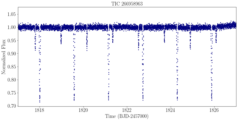
Planet Hunters NGTS: Potential Planet Candidates
Today, I presented the latest Planet Hunters NGTS results at the UK’s National Astronomy Meeting in the University of Warwick. Good news everyone! I am very excited to announce that we have four new planet candidates have been found by Planet Hunters NGTS. In addition, we have been able to get some observations of three of these new potential planet candidates with the Gemini South telescope in Chile!
I have spent the past several months developing a software pipeline to combine all of your assessments together for the various workflows that make up the website. This sifts through the candidates output from the NGTS algorithms to look for any new possible planets. In my preliminary search through the classifications available, I took the best candidates that were classified in the Secondary Eclipse Check and Odd/Even Transit Check and shared our findings with the rest of the NGTS team. Four of these candidates look like possible planet transiting planets and are shown in Figure 1.

There’s a lot of work that needs to be done to go from planet candidate to bonafide planet, so the four objects are still planet candidates. To confirm possible transit events requires using additional detection methods to get the mass of the orbiting body that confirm it has a mass less than a star or additional observations that can help statistically rule out the possible astrophysical false positives that can mimic planet transits (like eclipsing binaries). These candidates are around faint stars which will make validating these planets a tricky process.
Three of our planet candidates were observed in the past month to get follow-up observations. We worked with our collaborators in the US to apply for observing time on the Gemini South telescope. This involves: justifying why our candidates are interesting (there’s a lot of really interesting science that people want to do that we have to compete with!); justifying why the Gemini telescopes and Zorro instrument (see next paragraph) are the best tools for the job (in this case, Zorro is one of only a few instruments in the world that can carry out the kind of observation we need, another being ‘Alopeke on the Gemini North telescope in Hawaii); and calculating how much time we’d need to use the telescope for.
The instrument we are using is the ‘Zorro Speckle Imager.’ Zorro takes lots of images of the star in quick succession, which allows us to “freeze out” the effects of the Earth’s atmosphere that causes light from stars to be distorted (this effect is known as atmospheric seeing, see Figure 2). This allows us to spot whether there are any other stars so close to our targets that the NGTS telescopes couldn’t tell them apart. These background stars contaminate the light we measure for the main target star and dilute eclipsing binary light curves such that we can’t see the secondary transits, mimicking what we would observe for a true transiting planet. This isn’t a design flaw in NGTS but a reality of how different telescopes are built for different purposes. For example, Zorro isn’t designed to survey our targets for the long timespan, like NGTS has, in order to spot these transits in the first place. Using different telescopes for exoplanet follow-up and confirmation is much like a football (soccer) team: if the defenders don’t win the ball from the opposition (NGTS spotting transits), they can’t then pass it to the midfielders to move it up the pitch (Zorro checking for other stars).

Our observations were carried out by the excellent team of astronomers and support staff at Gemini and NASA a few weeks ago and we’re hoping to be sent the full final results soon.
What about the strikers in our analogy? If we find out that these targets are solo stars, that isn’t the final step in confirming an exoplanet (it’s also a big IF). We’d ideally take “radial velocity” measurements which allow us to measure the mass of the exoplanet. This technique works by detecting how much a star is “wobbling.” This wobbling is caused by the exoplanet orbiting the star and the amount of wobble relates to how much mass the exoplanet has. When we say the planets orbit the Sun, really we mean the planets AND the Sun orbit the entire Solar System’s common centre of mass. It just happens to be that this point is very close to the Sun since it’s so big. It’s the same story for exoplanets and their stars. The radial velocity measurements take the role of the striker in our analogy, although it’s important to say that this wouldn’t be the end of it and there’s still plenty other tests to do and data that we have to gather to confirm if any of these candidates are real exoplanets. If we’re unable to take radial velocity measurements then we can potentially use “multicolour photometry” to help towards validating the candidate. This involves checking whether the depth of the transit is the same when we observe the star with different filters on a telescope. These filters only let certain colours of light through, similar to how you’d mainly see pink if you wore Elton John’s famous tinted glasses. If there’s a difference in the depth then it suggests that there is a background eclipsing binary system that is mimicking the transit of an exoplanet. The difference in depth would be because stars have different colours depending on how hot they are, so if we see a shallower or deeper transit using a different filter it is because a background star isn’t as bright in that filter. For these four stars, getting radial velocity observations will be tough as they are very faint and would require lots of time on the world’s largest telescopes, but the first step is to see what the Zorro observations say. Once we can analyse and interpret the Zorro data, we will decide on the next steps.
It’s very exciting to have candidates. Even if we can’t confirm these candidates as official planets, just finding these is an important step. We can still use these planet candidates to estimate the rate of exoplanets around the stars observed by NGTS. Thank you to everyone who has contributed to our project so far, whether it’s been through classifying light curves or getting involved with discussing potential candidates and weird subjects on the Talk boards. We couldn’t have done this without you. Also thank you to the extremely helpful team of instrument scientists at Gemini who helped us to setup our observations and the team at NASA for processing our data.
We also have many more subjects from the Exoplanet Transit Search still to sift through with the Secondary Eclipse and Odd/Even Transit checks. I performed an initial search, so there is much more I will be doing in terms of analysis of the classification data over the next many months. I am very hopeful that there will be even more candidates to find! Stay tuned! We’ll keep everyone posted on the blog.
Triple star system found via Planet Hunters TESS
Exciting news alert! The Planet Hunters TESS community has helped identify another exciting system, this time comprised of zero planets and three stars. ‘Why is this a Planet Hunters TESS discovery?’ you may ask. Well, thirty thousand pairs of eyes visually looking at data collected by NASA’s Transiting Exoplanet Survey Satellite leads to many exciting discoveries- including asteroids, supernova, eclipsing binaries and multi-stellar systems – all of which have nothing to do with planets at all but are equally exciting! Our latest discovery is now available at https://arxiv.org/abs/2202.06964.

Why is TIC 470710327 interesting?
This latest discovery consists of three very massive stars (one of which is around 15 times more massive than our own Sun) orbiting around one another very rapidly – with two of the stars taking 1.1 days to orbit around one another and a third taking 52 days to orbit around the first two. While triple star systems are not rare, this one stands out due to the 52 day orbit star being more massive than the combined mass of the other two. This poses interesting questions regarding how this system could have formed. Did the two stars capture the third? Did all stars form much further out and spiral in towards one another to give us the compact configuration we see now?
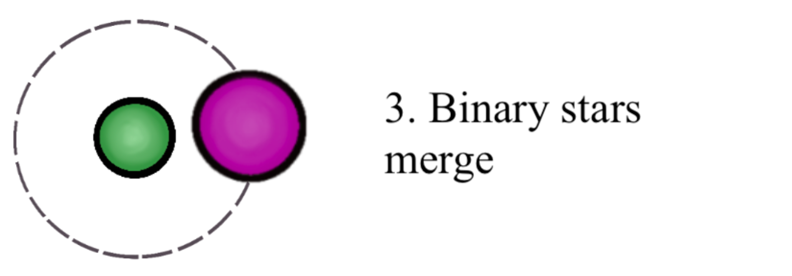
The future evolution of this system is equally interesting. Let’s look at what will happen to this system over the next couple millions of years. So this is where the system is now, two stars in an eclipsing binary with a third (more massive) star moving around it:

Now, as that outer star (purple one) continues to evolve its radius will expand, and it will likely expand in size so much that it will start to transfer mass over to the inner binary:

Which could mean that the two binary stars (the blue and yellow ones) could merge to become one star:
which will transform that triple systems that we had at the start into a binary (two star) system. However, eventually the outer star (the purple one) will run out of fuel and end its life as a supernova (the largest explosions in the Universe). The remnant of which is an extremely small and dense core of a star (called a neutron star).

Once the other star (the one that started off as two stars that merged into a single star) has run out of hydrogen to burn in its core, it will also start to expand in size. This will likely result in mass being moved over from the star (green) to the neutron star (black):

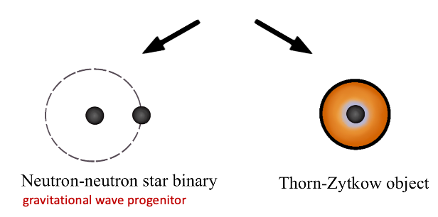
This brings us to the final and exciting stage in the evolution of this system! The former binary system (green) will also likely end its life by undergoing supernova and becoming a neutron star, which would leave us with a neutron-neutron star binary, which could eventually merge to cause a gravitational wave! Alternatively, the (first) neutron star could be completely engulfed by the other star, resulting in an exotic object called a Thorn-Zytkow object!! Either way, there’s an exciting future ahead of this system so stay tuned for the next couple of millions of years!
How did we study TIC 470710327?
Although this system has nothing to do with planets, many of the same tools and techniques used to characterise planets can also be applied to studying stars. For example, while planets show transit timing variations – slight delays in the expected times of transits due to other planets – stellar binary systems show the same effect when there is a third star nearby orbiting the two of them. Similarly, just as we can measure the masses of planets by looking at the doppler wobble in the host stars, we can study the masses of stars by studying their Doppler wobbles. As stars are much more massive, this effect is larger and therefore often easier to measure. Excitingly, we were able to study both of these effects in this new system in order to study its puzzling configuration.
Last but not least, I want to say a massive thanks to all of the Planet (and Star) Hunters taking part in the Planet Hunters TESS project! This is one of many interesting stellar systems that have been identified and I look forward to seeing what we find in the future. A special thanks to Safaa Alhassan, Elisabeth M. L. Baeten, Frank Barnet, Stewart. J. Bean, Mikael Bernau, David M. Bundy, Marco Z. Di Fraia, Francis M. Emralino, Brian L. Goodwin, Pete Hermes, Tony Hoffman, Marc Huten, Roman Janíček, Sam Lee, Michele T. Mazzucato, David J. Rogers, Michael P. Rout, Johann Sejpka, Christopher Tanner, Ivan A. Terentev and David Urvoy who are now coauthors of the discovery paper.
Planet Hunters NGTS German Translation
Today we have a guest post by Ruth Titz-Weider. Ruth is a researcher at the Institute for Planetary Research of DLR (German Aerospace Center) in Berlin.
We have translated the Planet Hunters NGTS website into German: Planetenjäger NGTS.
It’s ideal to bring real data of real exoplanet research to volunteers, students, and teachers in German speaking environments.
The Planets Hunters NGTS website is ideal to get people close to our exoplanet research activities at DLR, Institut für Planetenforschung, in Berlin. DLR has been supporting NGTS with the funding of eight cameras and is part of the scientific team. We are planning a teacher training before the summer holiday where we will use the Planet Hunters NGTS as a sort of hands-on-experiment.
False Positives: W-shaped transits

Computers are amazing, but sometimes they do something unexpected. In this blog post, we explain the reason you sometimes find a W-shaped transit on Planet Hunters NGTS.
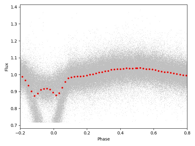
On Planet Hunters NGTS, we show you phase-folded light curves which are images produced by a computer algorithm that has calculated the best guess at the period of the transiting object (if there is one!). You can read more about how this is done in this blog post. However, sometimes the computer algorithm might calculate this period incorrectly. This can happen for a number of reasons but quite often it can be due to a deep secondary transit in an eclipsing binary system that the algorithm misinterprets as another primary transit. In the image below, the primary transits are the deep transits when the yellow star is completely blocked (occulted) by the redder star. The secondary transit is the shallower dip in the centre of the plot when the smaller star is blocking part of the large, red star. Note that this plot shows both the raw data points in grey and the binned data in red (explained below).

In the example above, the primary transits are at 0.5 and 3.0 days therefore the true orbital period is the difference between them, 2.5 days. If the computer correctly identifies this then you would be presented with an image zoomed in on the primary transit. However, if the algorithm doesn’t correctly notice the difference in depths then it may calculate the period to be 1.25 days, half of the true period, as it believes the shallow transit in the middle to be another primary transit. Once the algorithm has determined a period, it “bins” the raw data points (grey) to create the red data points. This means that we calculate the average flux of all the points in a set time window, which is referred to as a bin. Each red point in the plot above corresponds to a 30 minute bin and will contain around 140 raw data points on average since the NGTS telescopes take an image of the sky every 13 seconds. (The telescope cameras use 10 second exposures, followed by a 3 second delay before the next exposure while the shutter closes and the camera CCD reads out the flux on each pixel).
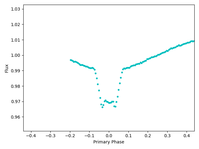
If the algorithm has folded the primary and secondary transit points on top of each other, as shown below, then the binning process will combine the raw fluxes into an average value somewhere in between the true flux values. This results in the erroneous W-shaped transit!
The next figure is an image from the Planet Hunters NGTS site that shows this W-shape, although it’s only a very slight effect. In this case, the subject gained enough votes to be pushed through to the odd/even transit depth check. This is expected since we yet don’t have a classification option for W-shaped transits.
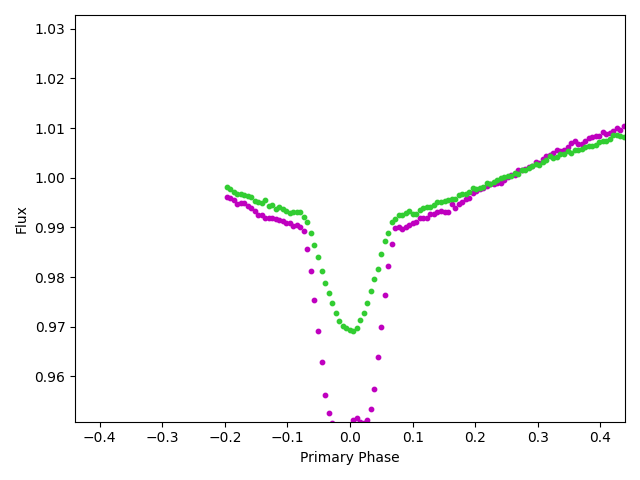
The odd/even transit check allows us to straight away spot the different depths of the primary and secondary transit. We can see that the magenta points correspond to the deeper primary transit while the green points show the shallower secondary transit. The distinct V-shape of both transits, as well as the rising flux after the transit are stereotypical of eclipsing binary systems.
If you spot something like this, then try to classify the shape of the transit as best you can into either U or V-shape. In the case of the example above, I’d choose V-shaped, but if you need more help then check out this blog post. Also, feel free to mark it as #w-shaped on the Talk channel, it helps us to check why this happens when our computer processes the data. Once we have analysed the rate at which this kind of transit shape occurs, we may introduce a W-shaped classification category to the interface, allowing you to more easily help us filter out these false positives.
Planet Hunters NGTS: Metadata
In this blog post, we explain the meaning of, and how to use, the different values and info given in the subject metadata on Planet Hunters NGTS.
On Planet Hunters NGTS, once you classify a subject you can choose ‘Done’ to move to the next subject and keep classifying, or you can choose ‘Done & Talk’ if you want to start a discussion with the Planet Hunters community about anything interesting you may have found. When you are looking at a subject image in the Talk discussion boards, you’ll be able to access the subject metadata by clicking the ‘i in a circle’ button. This metadata is additional info about the subject, some of which will be interesting to Zooniverse users wanting to delve deeper into their classifications.
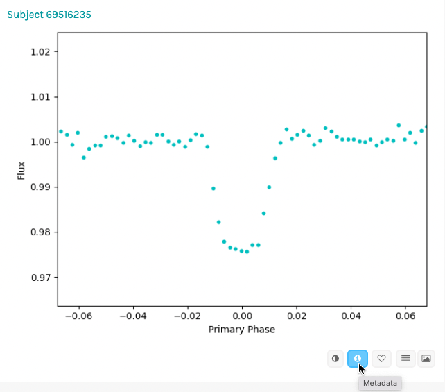
Once you click the metadata icon, you’ll find a varying number of information fields, depending on whether the subject has linked images or is a known planet, but more on that later.
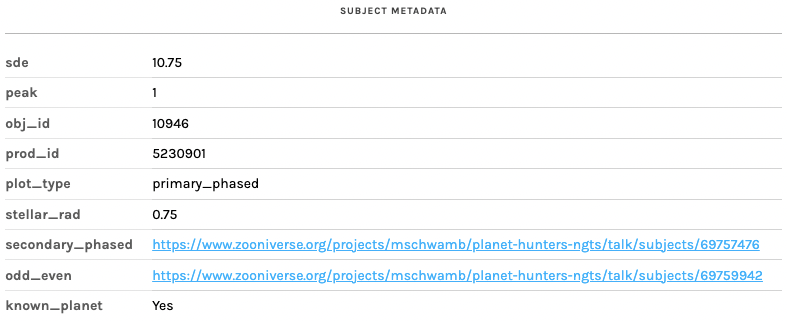
The first field is ‘sde’ which stands for ‘Signal Detection Efficiency.’ This value can be interpreted as how “strong” the signal is, according to the computer algorithm. The calculation of this value is described in Kovács et al. (2002) which describes the Box-fitting Least Squares (BLS) algorithm that forms the basis for the NGTS exoplanet transit searches.
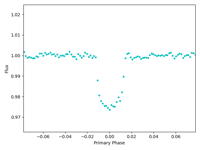
As a demonstration, consider a full light curve (not phase-folded) such as the image below (which uses artificial data). I’ve injected a transit with a 3-day period into the light curve and we’re going to use a BLS algorithm to search for this.
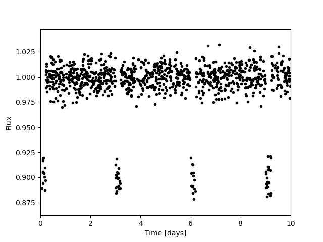
I’ve used the AstroPy package’s BLS periodogram tool. This calculates the ‘power’ for a range of periods, this ‘power’ is equivalent to our SDE value mentioned above. The resulting ‘periodogram’ is plotted in the figure below. This shows the power value plotted against period with peaks in the periodogram corresponding to where the algorithm believes there is a strong periodic signal in the light curve.
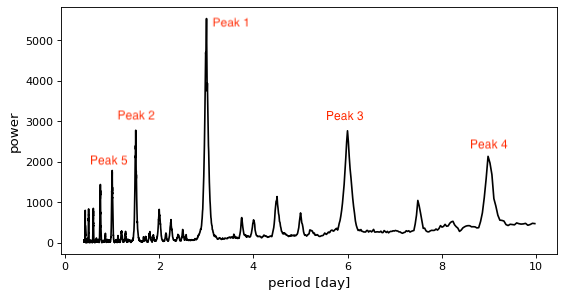
As we can see, the algorithm has picked out the strongest signal at a period of 3 days, just as we expected as this is the true period of the signal I injected. We also see peaks (of decreasing power) around 1.5 days, 6 days, 9 days and 1 day. You may notice that these are all multiples or fractions of the true period. We refer to these as period aliases and it’s expected that they will produce peaks in the BLS periodogram. Sometimes these can even be the true period of a signal, which leads us to our next metadata field.
‘peak’ is the strength of the peak according to the BLS algorithm, ranked by SDE. 1 is the strongest peak (our 3-day period in the example above), down to 5 for the 5th strongest. Anything less significant than this doesn’t have a phase-folded image generated for Planet Hunters NGTS. Currently only Peak 1 objects are on the Planet Hunters NGTS site as these are most likely to correspond to the true period of a transiting object but we plan to include plots for other peaks in future.
‘prod_id’ and ‘obj_id’ are internal identifiers that are used as labels for the stars. These values therefore only have meaning to the NGTS science team.
‘plot_type’ simply refers to which workflow this subject is from:
- ‘primary_phased’ is for subjects in the Exoplanet Transit Search. These plots show where we think the primary eclipse of the phase-folded light curve is. See Figure 1.
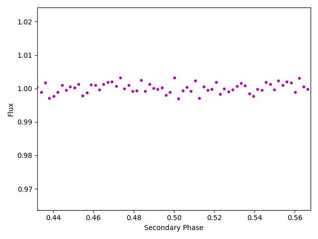
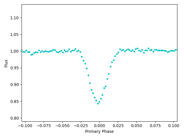
- ‘secondary_phased’ is for subjects in the Secondary Eclipse Check. These plots show where we think the secondary eclipse could be, around phase=0.5. See Figure 5 below
- ‘odd_even’ is for subjects in the Odd Even Transit Check. These plots show the odd (1st, 3rd, 5th, etc.) transits in green and the even (2nd, 4th, 6th, etc.) transits in magenta. If the depths of the odd and even transits don’t match then that’s a clear indicator that we’re looking at an eclipsing binary rather than an exoplanet transit. See Figure 6 below for the Odd/Even image corresponding to the subject shown in Figure 1.
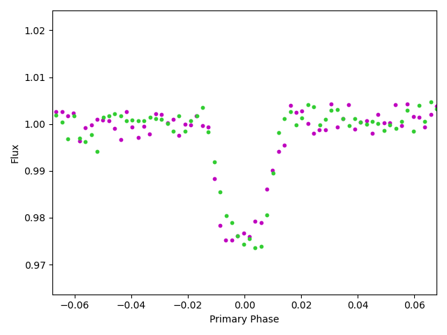
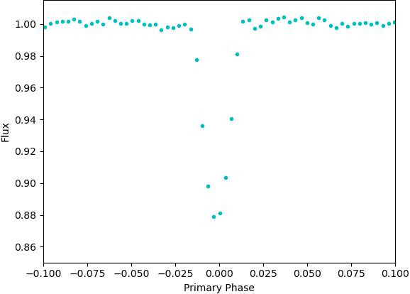
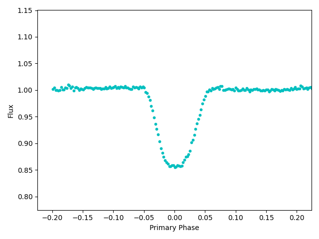
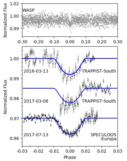
‘stellar_rad’ is the radius of the host star, expressed in units of Solar radii (i.e. a star with stellar_rad equal to 2.0 has a radius twice the size of our Sun). This can be used to estimate the radius of the transiting object. First, we estimate the depth of the transit. For the subject shown in Figure 1 (which is confirmed planet NGTS-5b), the transit depth is around 0.025 (or 2.5%), since the flux drops from 1.0 to 0.975 (typo corrected). We can then use this, along with the stellar radius of 0.75 Solar radii, in the equation:

to calculate an estimated planetary radius of 1.15 Jupiter radii. You can read more about how planet radius, stellar radius and depth are related here. The equation I use here is a quicker method as the multiplication factor of 9.73 is such that if you use R* in solar radii, as given in the metadata, then your answer will be in Jupiter radii. You can use this method to work out whether a transiting object is plausibly a planet, typically anything above 1.5 Jupiter radii is unlikely to be a planet.
(Note sometimes the stellar radius value will say ‘nan’ or ‘unavailable,’ this just means we don’t have a good measurement of the star’s radius.)
Extra fields
‘primary_phased,’ ‘secondary_phased’ and ‘odd_even’ provide links to the different plot types for subjects that have passed into the secondary and odd/even workflows. This makes it easier to vet candidates as you can view all the available data quickly and easily.
Finally, we have the ‘known_planet’ field. This will only appear for previously known exoplanets (such as NGTS-5b above) and means that the subject image you are viewing corresponds to a planet that appears in the NASA Exoplanet Archive. Finding known exoplanets is a useful test of the detection efficiencies of the project as a whole, and it’s always exciting to know if you’re looking at data from a real exoplanet system too! Some subjects on the Planet Hunters NGTS site are still undergoing follow-up by the NGTS science team so might be strong planet candidates but won’t be confirmed and published exoplanets. This means that there will be subjects not marked as known planets in their metadata, but the NGTS team may already be aware of it and have put in the work to begin characterising the system further.
We hope this blog post can serve as a useful reference in future as you get involved with Planet Hunters NGTS.
U- or V-shaped dip? How to spot the difference?
When searching for exoplanets, the shape of the transit can tell us a lot about what object we could be looking at. For the Planet Hunters NGTS exoplanet transit search, we ask you to identify if a transit is U-shaped or V-shaped, as well as whether there’s stellar variability, data gaps or no significant dip in the flux at all. An exoplanet transiting a star will typically produce a U-shaped dip, but there are situations where that isn’t the case (more on that below). Meanwhile an eclipsing binary (two stars orbiting each other) will produce a V-shaped dip most of the time.
The first plot (Figure 1) shows a clear V-shape produced by an eclipsing binary system. In this case, the transiting star only partially eclipses the target star, meaning that it passes across the edge of the disk of the target star but never passes fully in front. This means that the point of minimum flux doesn’t last long before the flux starts to increase again.
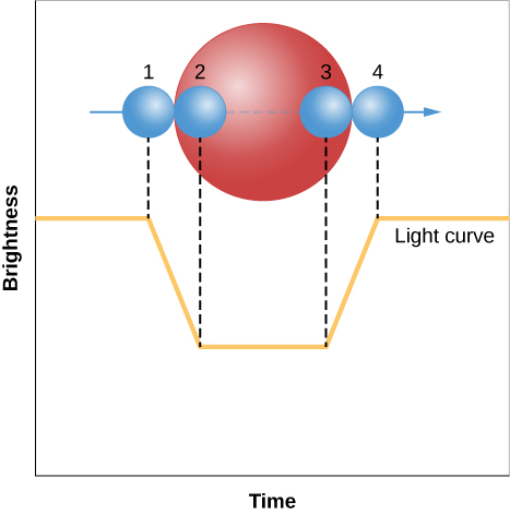
The defining difference between U- and V-shaped dips is the angle of the sides of the transit, or ingress and egress to give them their scientific names. Ingress is when the transit begins and the flux is decreasing to the minimum (position 1 to position 2 in Figure 2), while egress is when the transit is ending and flux starts to increase back to the normal level (position 3 to position 4 in Figure 2).
V-shaped dips have sides that are at an angle whereas U-shaped transits will have a steeper decrease and increase in the flux, so much so that the sides of the transit will be almost vertical. The reason V-shaped dips have angled sides is because the object blocking out the light is typically (but not always!) another star. The eclipsing star is large (compared to a planet) so takes more time to pass fully in front of the target star, therefore the decrease in flux happens over a significant time period and we get an angled ingress (likewise for the egress as the star stops blocking light).
The angled sides are more pronounced in Figure 1, but don’t be fooled by dips with a curved base like Figure 3 below! If the transit has angled sides then it’s still a V-shape! The curved base of the transit is caused by a phenomenon called ‘limb darkening,’ where the central disk of a star appears brighter than the edge. The eclipsing star in this system is not just grazing the limb of the target star either, which is why the minimum flux of the transit is sustained for a range of phases.
How vertical is vertical? Sadly there isn’t a clear answer to this, which is why we use human vetting rather than just a computer to check these light curves. The example below (Figure 4) is the light curve for confirmed exoplanet HATS-43b, which was classified as U-shaped by all 20 volunteers who viewed it. This is a clear example of the near vertical drop in flux for the sides of the transit. The small radius of the planet compared to its host star means that it almost instantly passes through the ingress and egress phases, compared to the time taken by a larger star in an eclipsing binary system.
But wait! V-shaped dips can still be exoplanets too! Just like the partial eclipse that produced the sharp, V-shaped dip in Figure 1, an exoplanet can perform a grazing transit where it just crosses the limb of the star and doesn’t go over the centre of its host star’s disk. This will produce a very shallow V-shaped dip, therefore we will get round to searching these classifications for potential exoplanets too! The sides of the dip appear more angled due to the shorter total duration of a grazing transit; it’s very likely that the scale of the x-axis on the plots (the phase) will show a much smaller range of numbers due to how short these transits will be. The ingress and egress times will be similar to a regular transit but the central dip is much shorter. The limb darkening effect also has a more obvious effect on the shape of the dip, which we can see in the light curves below for a near-grazing transit by WASP-174b (Figure 5). The dip has angled sides due to the zoomed in x-axis and has a curved base due to limb darkening. This is a classic curvy V-shape, but it’s also a real exoplanet!
There isn’t a definitive answer for when a curvy V becomes a regular U-shape, but as always your intuition and best guess is what we want! We hope this blog post makes it easier to spot the differences between U- and V-shaped dips when you’re classifying light curves on the Planet Hunters NGTS site, and remember you can always check the Field Guide or ‘Need some help with this task?’ for more help. There’s also the team of researchers and moderators on the ‘Talk’ forums who will be happy to help!
Sean & the Planet Hunters NGTS Team
Welcome to a new Planet Hunters!
We’re extremely happy to welcome a new member of the PlanetHunters family. Planet Hunters: NGTS is our first project using data from a ground based survey – the Next Generation Transit Search based at Paranal in the Atacama Desert in Chile.The twelve telescopes of NGTS aim to find planets around the brightest stars; the hope is that, unlike the large number of planets found with NASA’s Kepler, which provided data for the original Planet Hunters, these will be targets that can be followed up with further observations designed to characterise their mass, composition and atmospheres.

As with the Exoplanet Explorers project we ran on Zooniverse a while back, the aim of this new project is to review candidates that have been selected by automatic searches. The hope is that this will make our hit rate higher, but it does mean the task is a little different. The project lives on its own webpage as ngts.planethunters.org, and is led by Meg Schwamb, Chris Watson and Sean O’Brien at Queen’s University Belfast, along with their colleagues. They’ll be responsible for looking at your data, with the help of the Planet Hunters:TESS team.
With this new project there should be enough data to keep you all searching for more than the few days each month TESS data is available. Happy hunting!
(Image: the NGTS telescopes in Paranal, with ESO’s Very Large Telescope visible in the background).
Planet Hunters TESS finds an exciting two-planet system
We have some exciting news – you helped discover another exciting planet system: TIC 349488688 (also known as HD 152843). This exciting discovery follows on from our validation of the long-period planet around an evolved (old) star, TOI-813, and from our recent paper outlining the discovery of 90 Planet Hunters TESS planet candidates, which give us encouragement that there are a lot more exciting systems to be found with your help!
The new exoplanetary system, TIC 349488688, consists of two planets that are similar in size to Neptune and Saturn in our own solar system, orbiting around a bright star that is similar to our own Sun. Planet b is around 3.4 times the size of the Earth, and takes around 12 days to complete an orbit around the star. The outer planet, planet c, is around 5.8 times the size of the Earth and has an orbital period somewhere in the range of 19 to 35 days. The paper has been published by the Monthly Notices of the Royal Astronomical Society (MNRAS) journal and you can find a version of it on arXiv at: https://arxiv.org/abs/2106.04603

Figure 1: the arXiv version of the published paper.
Multi-planet systems, like this one, are very exciting as they offer a wealth of information. In particular, they allow for comparative planetology: the study of two planets that necessarily formed at the same time and out of the same material, but which have evolved in different ways over time resulting in different planet properties that we observe today. Studying these two planets together, therefore allows us to test theories of planet formation and evolution.
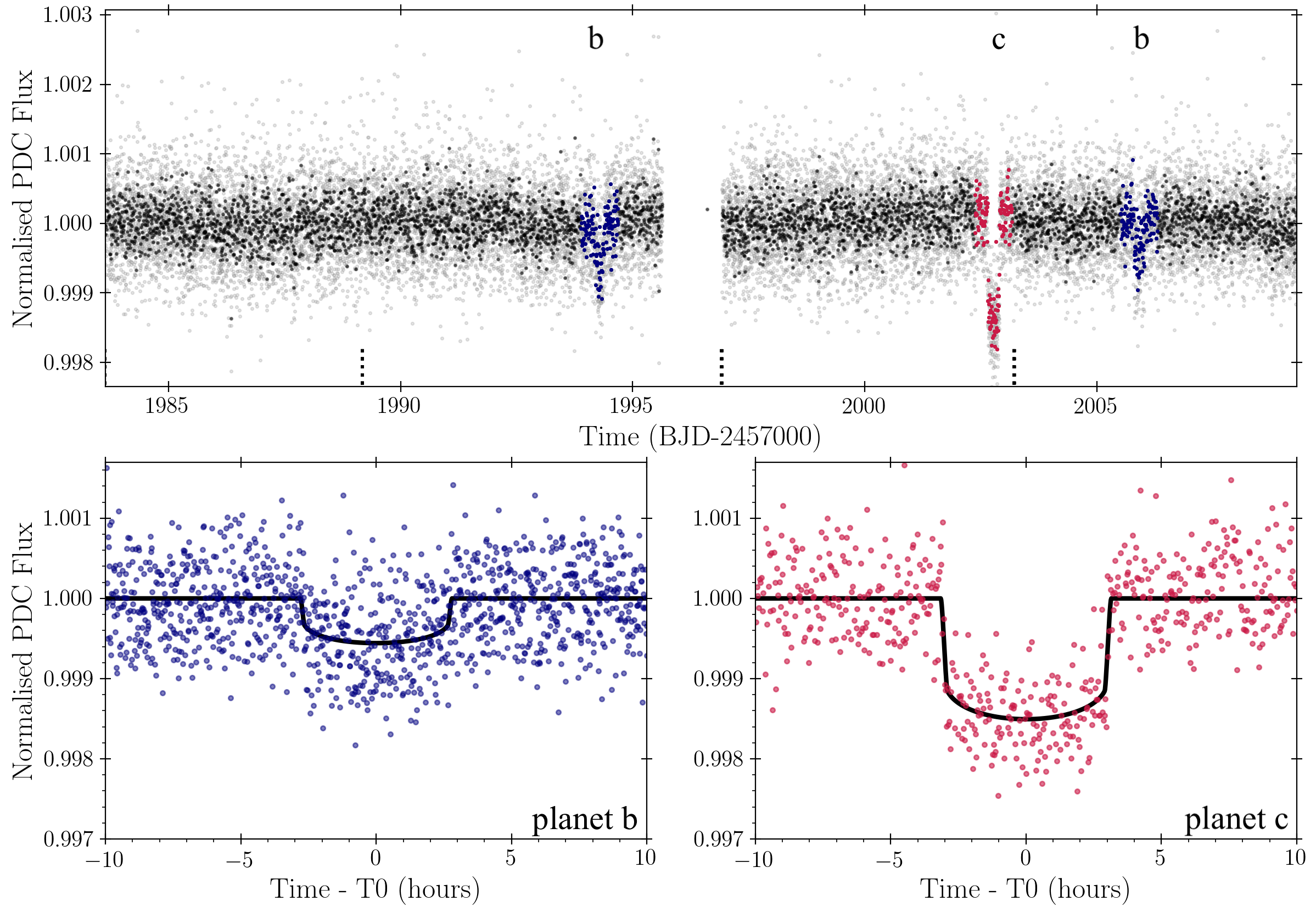
Figure 2: TESS lightcurve showing the transits of planet b in blue and the single transit of planet c in pink.
Detection and Validation of the planets
The target was observed in Sector 25 of the TESS data only and the light curve displayed three transit events belonging to the two different planets (see Figure 2). These events were flagged on the talk discussion forums and brought to the attention of the PHT science team. Once it was flagged, we ran a large number of vetting tests to validate it as a planet. First, we made sure that the signal wasn’t caused by a jolt in the TESS satellite or a background event. Next, we ruled out ‘astrophysical’ false positives – signals caused by other astrophysical phenomena such as two stars orbiting around one another, known as an eclipsing binary.
Follow-up Observations
After ruling out a large number of astrophysical and instrumental false positive scenarios, we were confident that the signals were real! However, in order to truly confirm a planet you have to measure its mass. One of the ways to do that is to use what is known as the radial velocity method. As a planet orbits around it’s host star, the gravitational pull between the two bodies causes the star to ‘wobble’ back and forth, meaning that the star is sometimes moving towards us and sometimes moving away from us. As the star moves towards us, the light that it gives off is ‘squished’ and appears more blue, whereas when it’s moving away from us the light is ‘stretched’ and appears more red. The amount of these red and blue shift scales with the mass of the planet.
In order to measure these red and blue shifts we used two ground-based telescopes: HARPS-N located in La Palma, Canary Islands; and EXPRES located at Lowell Observatory, Flagstaff, Arizona. These two telescopes allowed us to obtain spectroscopic observations – observations that split the light of the star up into its individual wavelengths, similar to how a prism splits light into a rainbow. Careful analysis of this split light allowed us to detect the tiny shifts from red to blue and back to red, which were caused by the two planets orbiting around TIC 349488688. We obtained enough racial velocity measurements to estimate the mass of planet b to be around 12 times more massive than the Earth, and to place an upper mass limit of 28 times the mass of the Earth on planet c.
Why is this system so interesting?
Even though there are now hundreds of confirmed multi-planet systems, the number of multi-planet systems with stars that are close enough such that we can observe and study them using ground-based telescopes remains exceedingly small. The proximity and brightness of HD 152843 is one of the properties that makes this new system stand out. To date we have been able to constrain the masses of the two planets and we are currently continuing to monitor the system to confirm them.
The masses that have already been derived suggest that both planets have low densities, and therefore are likely to have extended gaseous atmospheres. Combined with the brightness of the stars these properties offer exciting prospects for probing the atmospheres and chemical composition of both planets in the future, for example with upcoming space telescopes such as NASA’s James Webb Space Telescope.
Last but not least this system is interesting because it was discovered by you! With this find you have once again shown that with visual vetting we are able to detect exciting planet systems that the automated computer algorithms struggled to find. Thank you to everyone who helps out with the search for distant worlds on Planet Hunters TESS and who help to further our understanding of our Galaxy. A special thanks also to Safaa Alhassan, Elisabeth M. L. Baeten, Stewart J. Bean, David M. Bundy, Vitaly Efremov, Richard Ferstenou, Brian L. Goodwin, Michelle Hof, Tony Hoffman, Alexander Hubert, Lily Lau, Sam Lee, David Maetschke, Klaus Peltsch, Cesar Rubio-Alfaro, Gary M. Wilson who are now coauthors of the discovery paper.
Planet Hunters TESS II: results from the first two years
We have some very exciting news: our paper summarising the results from the first two years of Planet Hunters TESS has been accepted for publication! Check out the paper here.
The paper outlines the ins and outs of planet Hunters TESS project and presents 90 new planet candidates from the first two years of the TESS mission (sectors 1 to 26). These planets wouldn’t have been found without the help of all of the citizen scientists taking part in the Planet Hunters TESS project. The paper includes a link to a site that lists all of the citizen scientists who identified each of these 90 planet candidates mentioned in the paper. This page can also be found here.
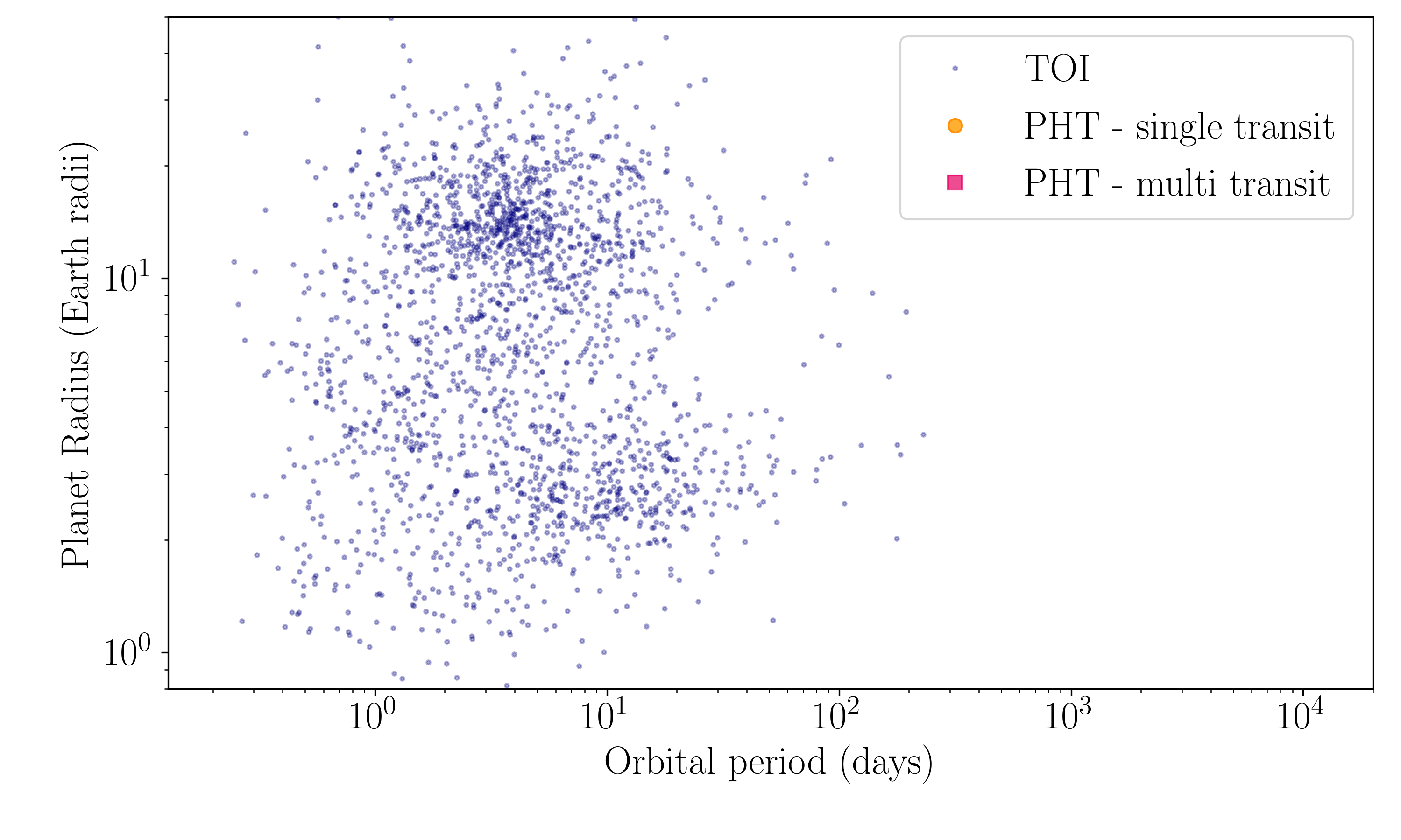
The majority (81%) of the planet candidates outlined in the paper only exhibit a single transit event in the TESS lightcurve, meaning that they tend to have longer orbital periods (where the orbital period corresponds to the duration of a ‘year’ on this planet) than the average duration of the planets found by the TESS automated algorithms. This is because automated pipelines often require two or more transit events in order to be able to detect the signal. However, with visual vetting, we are equally sensitive to a single transit event as we are to planets that transit multiple times within the duration of one light curve.
You can see that in the figure below, where the orange and pink points show the PHT candidates, and the blue points show the automated pipeline found Tess Objects of Interest (TOIs). The figure highlights that the planets identified with PHT tend to have longer orbital periods than the TOIs, and therefore allowing us to study the characteristics of a different ‘set’ of planets, and maybe even of planets that are more similar to the planets within our own solar system.

Even though the majority of the planet candidates outlined in the paper are not yet confirmed planets, we are following them up using ground-based telescopes which are situated around the world, including in Australia, Chile, USA and the Canary Islands. Hopefully these observations, including both photometric and radial velocity observations, will allow us to confirm the planetary nature of these objects, and even derive masses for some of them which will allow us to infer their densities and therefore bulk compositions. This is ongoing work and we hope to share some of it with you in the near future.
In addition to the 90 new planet candidates, the paper presents some of the most interesting stellar systems that have been discussed on the Planet Hunters TESS Talk discussion forum. An example of a potential multi stellar system is shown below.
Multi stellar systems not only provide very interesting and pretty lightcurves, they also allow us to probe stellar evolution theories in more detail, as all the stars in one system must have necessarily formed at the same time and out of the same material. This highlights some of the other exciting science that results from Planet Hunters TESS and from the continued work of so many citizen scientists.
Since the launch of the Planet Hunters TESS project, almost exactly 2 years ago, we have had over 25.5 million classifications completed by over 25 thousand citizen scientists from around the word. This huge global effort can help us understand what kind of planets exist within our galaxy, how planets form and evolve over time, as well as bring to light some of the other interesting and bizarre astrophysical phenomena that TESS observed over the last two years.
